This work was done while working as a PhD student at the University of Nevada, Reno, supervised by Mark Lescroart.

Encoding models are a powerful approach to measuring whether different parts of the brain respond to different features. Cortical regions that (linearly) respond to a set of features should be predicted accurately by an encoding model trained on those features, whereas regions unrelated to those features are predicted poorly. For example, I used encoding models as the foundation of my project exploring body-part selectivity, and the DNN-based simulation models I’ve been using are themselves a form of encoding models.

However, a core challenge when using encoding models is distinguishing between true selectivity for the features of interest and selectivity for other features are correlated with those features in your stimuli. For example, bodies in natural videos tend to appear at predictable locations in the visual field (legs at the bottom, heads near the top), so an encoding model fit on on ‘leg’ features will also predict well in early visual cortex that is selective for the lower visual field. This makes it hard to tell whether a voxel is actually selective for the features we’re studying.

The standard tool for handling this is variance partitioning, where you construct sets of possible correlated features and additional encoding models them, and compare the results. This works well if you know beforehand what all of the correlated features are, and have a way to quantify them in your stimuli. But in any situation where this isn’t the case (which I think is probably most of the time), we need something better.

Solution: Compositional Feature Mapping

I developed an approach I call Compositional Feature Mapping (CFM) to leverage this. Rather than fitting an encoding model directly from features to brain responses, CFM constructs the mapping by combining two separate models. First, it fits a linear regression mapping the features of interest F (in this case, body location features) to DNN activations A extracted from the same stimuli:

\[\mathbf{A} = \mathbf{F} \mathbf{W}_{F \rightarrow A}\]

Second, it uses the previously fit DNN-to-brain mapping that predicts brain responses B from these DNN activations:

\[\mathbf{B} = \mathbf{A} \mathbf{W}_{A \rightarrow B}\]

By multiplying these two sets of weights together, CFM creates a complete mapping from the features of interest to brain responses:

\[\mathbf{B} = \mathbf{F} \mathbf{W}_{F \rightarrow A} \mathbf{W}_{A \rightarrow B}\]

CFM addresses the issue of correlated stimulus features by using DNN activations as an intermediate feature space. So why does this help? This comes from the idea that the internal features learned by vision DNNs are a set of ‘universal features’. Multiple lines of work suggest that DNNs converge toward similar representations that turn out to be useful across a wide range of tasks: generic activation features from pretrained CNNs transfer well to novel recognition tasks, self-supervised models learn representations comparable to fully supervised ones, and the Platonic Representation Hypothesis argues that representations across different models, modalities, and training objectives are converging toward a shared statistical model of the world.

By first fitting an encoding model mapping brain responses to these features, brain responses that are better explained by correlated features can be ‘absorbed’ by the DNN activations that actually represent those correlated features. And voxels that actually respond to the features we’re interested in will be mapped to DNN activations that really represent these features. By then multiplying by weights mapping from our features of interest to the DNN activations, we’re essentially ‘filtering’ out selectivity for correlated features.

This can be (loosely) thought of as similar to doing variance partitioning with all plausible alternative sets of features.

Example: Body Part Selectivity

As a concrete example, I applied CFM to a set of body-location features, the same set of features I used in previous work studying visual processing of body parts. These features consist of 15-by-15 spatial maps representing the presence of different body parts (heads, trunks, arms, hands, legs, and feet) in the visual field. I extracted these features from a set of naturalistic video clips, and fit both a standard encoding model and a CFM model to map these features to recorded brain (fMRI) responses to the same video clips.

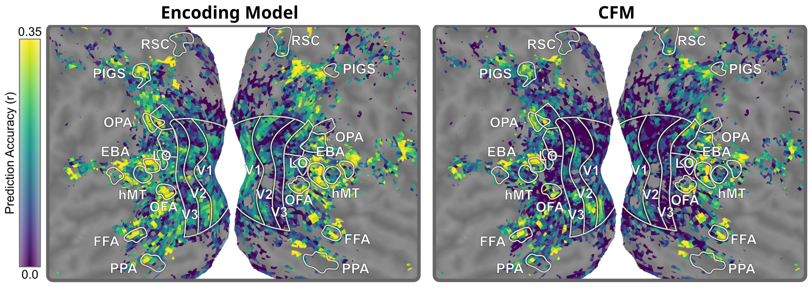
Shown below, both the encoding model and the CFM model accurately predict brain responses in various parts of the brain. This includes high prediction accuracy in known body-selective regions including EBA, OFA, and FFA. However, the encoding model also yield high prediction accuracy in regions known to not be body-selective, such as early visual areas V1, V2, and V3. If we trusted the encoding model, we would conclude that these regions are just as body-selective as actual body-processing regions.

We can also look at the weights of the CFM model, which dictate the mapping from features to brain responses. Looking just where these weights are high (red), we find patches of strong selectivity in only a few spots: EBA, OFA and FFA, and pSTS (another known body-procession area). Unlike standard encoding models, CFM excels at specificity–it only highlights areas that are really selective for the features being studied.

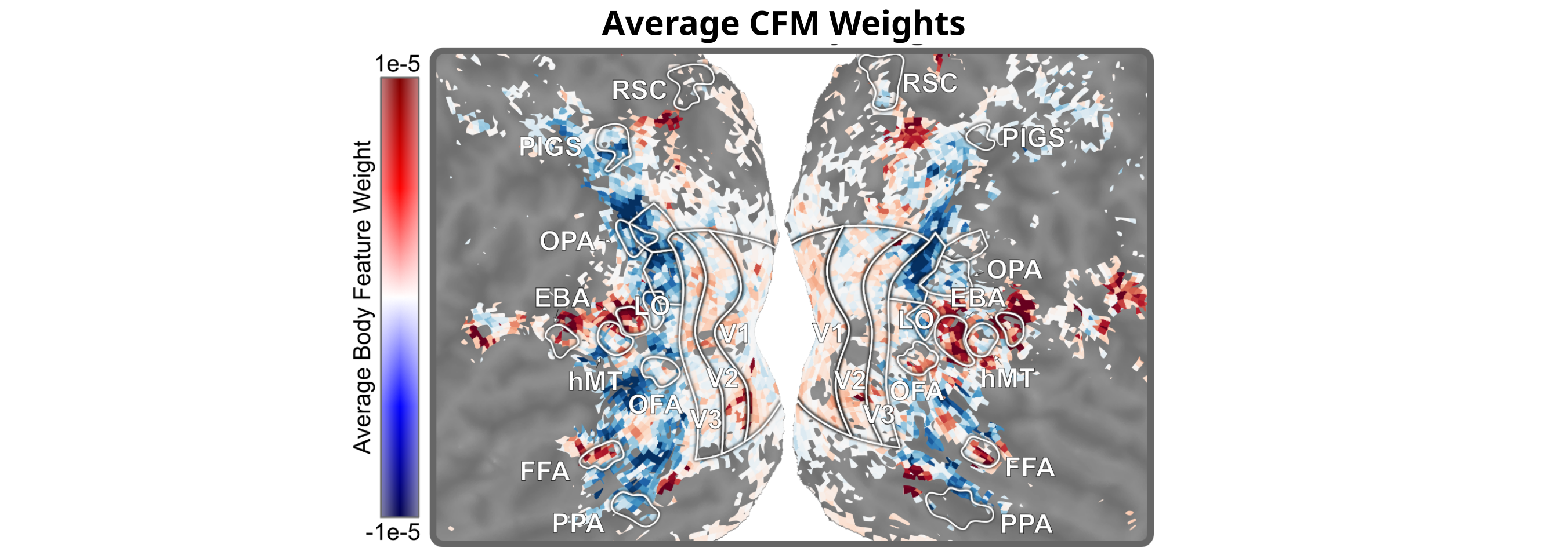
Side note: if you look closely at the above figure, you might notice two other smaller patches of red in each hemisphere: one located adjacent to RSC (near the top of the figure), and one adjacent to PPA (near the bottom of the figure). Both RSC and PPA are considered scene-processing regions, so what’s going on here?

(Hint: see Discovering New Body-Selective Brain Regions.)

For more details and results, see Chapter 2, Section 2.3.3 (“Fitting Encoding Models on Simulated Responses”) of my dissertation.